Background

True distribution

Assumption

Given \(N\) training examples \((\vec{x}_1, y_1), \cdots, (\vec{x}_N, y_N)\) where \(\vec{x}\) is feature set and \(y\) is label. Assume each features follow independent and identically distribution (i.i.d.) We have

\[(\vec{x}_i, y_i) \sim p^*\]

Classification Problem

Classifier

A classifier is a function \(h\), mapping feature vector \(\vec{x}\) to label \(\hat{y}\).

For sample \(\vec{x}_i\) the classifier returns predicted label \(\hat{y}_i = h(\vec{x}_i)\)

Goal

A learning algorithm takes a dataset and returns a classifier \(h\).

True Error

The true classification error of \(h\) is

\[\begin{gather} \mathbb{P}[Y \ne h(X)] = \mathbb{E}_{X, Y \sim p^*} [ \mathbb{1}(Y \ne h(X)) ] \\\\ \mathbb{1}(X) = \begin{cases} 1 & X = True \\ 0 & X = False \end{cases} \end{gather}\]

Where \(\mathbb{1}\) is the indicator function

It evaluates the average number of misclassifications on a very large test set.

Bayes optimal

A classifier \(h^*\) which minimizes the true classification error is called Bayes optimal

Let \(p^*(X, Y)\) be the unknown data generating distribution. The classifier

\[h^*(x) = arg \max_{y} p^*(y|\vec{x})\]

It means we need to know the prior probabilities ahead and then to determine the class of \(y\) that has highest probability.

KNN

Label new point according to closest training points.

• Label a new point according to majority vote of its $k$ nearest neighbors
• Stabler decision, averages data noise
• For binary classification, $k$ should be odd
• Theoretically sound

if

1. number of training points \(N \rightarrow \infty\)
2. number of neighbors \(k \rightarrow \infty\)
3. \(N\) grows quicker than \(k\) \(\frac{k}{N} \rightarrow 0\)

Then KNN converges towards the Bayes optimal classifier

KNN needs a distance metric

basically, it is Euclidian norm.

Naive Bayes

Bayes Rule

\[p(A|B) = \frac{p(B|A)p(A)}{p(B)}\]

For vector, it converts to

\[p(y|\vec{x}) = \frac{p(\vec{x}|y)p(y)}{p(\vec{x})} = \frac{p(\vec{x}|y)p(y)}{\sum_{y} p(\vec{x}|y)p(y)}\]

Since \(p(y \vert \vec{x}) \propto p(\vec{x} \vert y ) p(y)\) , \(p(\vec{x})\) is not necessary.

Naive Bayes Assumption

Assuming conditional independence of the features. Then, we have

\[p(\vec{x}|y) = \prod_{d=1}^{D} p(x_d|y)\]

Naive Bayes Classifier

Let \(p(y)\) be an estimate of the true class proportions \(p^* (y)\), and \(p(x_d \vert y )\) estimates of the true class-conditional distributions \(p^*(xd \vert y )\), for each feature \(X_d , d = 1 . . . D\).

The Naive Bayes Classifier is given as

\[h_{NB}(\vec{x}) = arg \max_{y} p(y) \prod_{d=1}^{D} p(x_d \vert y)\]

Laplace smoothing

for feature \(x_d\) in all features \(\vec{x}\), it has \(K\) choices. \(x_d \in \{1, \cdots, K\}\). then the Laplace smoothing is

\[p(x_d = f | y = c) = \frac{\mathbb{1}(x_d = f, y = c) + \alpha}{\mathbb{1}( y =c ) + \alpha K}\]

\(\mathbb{1}(x_d = f, y=c)\) is the number of data items that \(x_d = f\) and \(y = c\) in the whole dataset.

Since each feature follows i.d.d. we have

\[p(\vec{x} = \vec{f} | y = c) = \prod_{i=1}^{d} p(x_i = f_i | y = c)\]

According to the Bayes Rule, we have

\[p(\vec{x} =\vec{f}) = p(y = c) \prod_{i=1}^{d} p(x_i = f_i | y = c)\]

The generally idea to use smoothing is that in some case, the value of \(\mathbb{1}(x_d = f, y=c)\) might be \(0\) if it is not occurred in the dataset, leading to an incorrect probability distribution.

Therefore, we add smoothing parameter to both numerator and denominator to force it greater than \(0\).

log-domain

Since the value of a probability is in \([0, 1]\), therefore, the value of \(p(\vec{x} = \vec{f})\) will be too small to calculate and store in the computer.

Therefore, instead of store the original value, we can store it in the log-domain and compute. Then we have

\[\log p(\vec{x} = \vec{f}) = \log p(y = c) + \sum_{i= 1}^{d} \log p(x_i = f_i | y = c)\]

Generally, the base is \(e\).

Decision Trees

Given a set of features \(X_1, X_2, \dots , X_D\) (discrete or continuous) and a class variable \(Y\), a Decision Tree is a directed binary tree with two types of nodes:

• Decision nodes (internal nodes) Decision nodes are associated with a feature \(X_i\) and a boolean function \(f: X_{i} \mapsto {true, false}\)
• Prediction nodes (leaves). It associated with either
  • a fixed label \(y\)
  • a distribution over labels \(p(Y)\)

Training Methods

CART

L0 <- all nodes
for
	L1, L2 = split(L0)
	L0.left = L1
	L0.right = L2

	split(L0.left)
	split(L0.right)
end

function split(L)
	for possible decison Xd do
		 cost(Xd, f)
	end

	return Xd with min cost
end

function cost(Xd, f)
	N0 <- number of data points to L0
	N1, N2 <- number of data points to L1, L2

	cost = (N1/N0)*impurity(L1) + (N2/N0)*impurity(L2) - impurity(L0)
end

Stopping Criterion

• Too small improvement of cost
• Too few data points They are both called threshoulds.

Impurity Measures

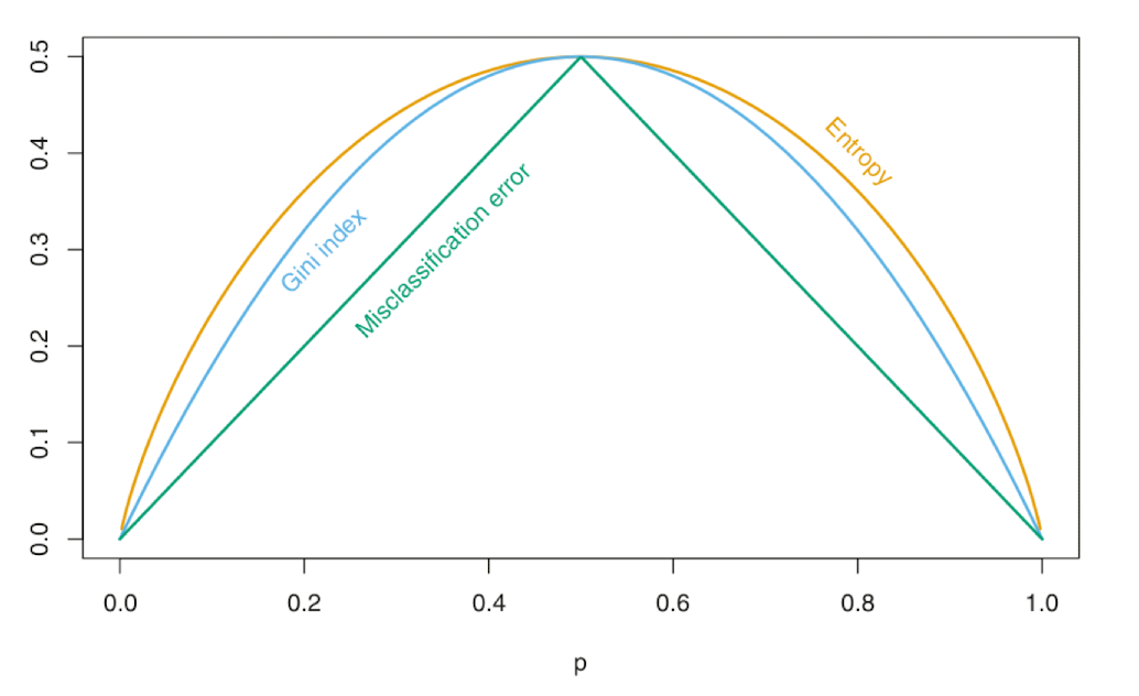
Gini Impurity

\[G = 1 - \sum_{y} p^2(y)\]

Entropy

\[E = - \sum_y p(y)log(p(y))\]

Self-Classification Error

\[C = 1 - \max_y p(y)\]

Random Forests

Improve performance of Decision Trees by Bagging algorithm to reduce the variance

• Make \(K\) bootstraps
• Train \(K\) classifiers, one for each bootstrap
• Aggregate the result: Averaging, majority vote…..

Bootstrap

Given \(N\) samples, generate \(K\) new datasets of size \(N\) by sampling with replacement, which are called bootstraps.

For large \(N\), each bootstrap contains only \(1 - \frac{1}{e} \approx 63.21\%\) of the original samples.

originSet = [x1, ... , xn]

for i in 1..k
	for j in 1..n
		bootstrap[i][j] = originSet[random(1, n)]
	end
end

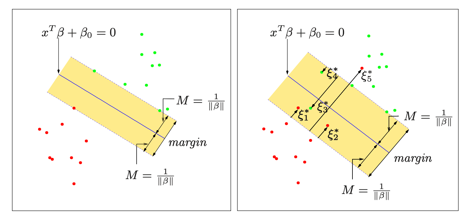
SVM

Build a hyperplane and max margin.

A hyperplane can be represented in vector form:

\[\begin{gather} \vec{x}^\intercal \vec{\beta} + \beta_0 = 0 \end{gather}\]

Therefore, it converts to an optimization problem:

\[\max_{\vec{\beta}, \beta_0} \min_{i} \frac{y_i(\vec{x}_i^\intercal \vec{\beta} + \beta_0)}{\lVert \vec{\beta} \rVert}\]

It means maximize the min distance between every point to the hyperplane

But this is not a convex function. Therefore, we try to make it convex by introducing the margin hyperplanes:

\[\begin{gather} \vec{x}^\intercal \vec{\beta} + \beta_0 = 1 \\ \vec{x}^\intercal \vec{\beta} + \beta_0 = -1 \\ \end{gather}\]

Therefore, the distance between the hyperplane and the margin hyperplane is \(\frac{1}{\lVert \vec{\beta} \rVert}\)

Therefore, the optimal question converts to

\[\begin{gather} & \max_{\vec{\beta}, \beta_0} \frac{1}{\lVert \vec{\beta} \rVert} \\ s.t. & y_i(\vec{x}_i^\intercal \vec{\beta} + \beta_0) \ge 1 \end{gather}\]

Then we can convert it to convex easily to:

\[\begin{gather} & \min_{\vec{\beta}, \beta_0} \frac{1}{2} \lVert \vec{\beta} \rVert^2 + C \sum_{i} \xi_i \\ s.t. & y_i(\vec{x}_i^\intercal \vec{\beta} + \beta_0) \ge 1 - \xi_i \\ & \xi_i \ge 0 \end{gather}\]

We square \(\beta\) to make it differentiable everywhere.

We introduce \(\xi\) to tolerant non-separable data.

Then, we can use Lagrangian Relaxation and Lagrangian Duality to solve it.

\[\begin{gather} & L_P(\vec\lambda, \vec\mu) = \min_{\vec{\beta}, \xi} \frac{1}{2} \lVert \vec{\beta} \rVert^2 + C \sum_{i} \xi_i - \sum_{i} \lambda_i (y_i(\vec{x}_i^\intercal \vec{\beta} + \beta_0) - (1 - \xi_i)) - \sum_{i} \mu_i \xi_i \\ \\ & L_D^* = \max_{\vec{\lambda}, \vec\mu} L_P \\\\ \end{gather}\]

use the Primary constraints to eliminate the primal variables

\[\begin{gather} \nabla_{\vec{\beta}, \beta_0, \xi_i} L_P = 0 \Rightarrow \begin{cases} \vec{\beta} = \sum_{i} \lambda_i y_i \vec{x}_i \\ \sum_{i} \lambda_i y_i = 0 \\ \lambda_i = C - \mu_i \end{cases} \\ \\ \Rightarrow L_D = \sum_{i} \lambda_i - \frac{1}{2} \sum_{i,j} \lambda_i \lambda_j y_i y_j \vec{x}_i^\intercal \vec{x}_j \end{gather}\]

Then we can use Kernel trick

Kernel Trick

For \(L_D\), it is all about \(\vec{x}^\intercal \vec{x}\), the inner product of vectors. we can treat it as a kernel

\[K_{ij} = \vec{x}_i^\intercal \vec{x}_j\]

We can convert our boundary to non-linear function: \(y_i = h(\vec{x}_i)^\intercal \vec{\beta} + \beta_0\)

Then the kernel is changed in the same way:

\[K_{ij} = h(\vec{x}_i)^\intercal h(\vec{x}_j)\]

Therefore, for high-enough feature space, the data will be separable. Then the objective converts to

\[\begin{gather} & \max_{\lambda} L_D = \sum_{i} \lambda_i - \frac{1}{2} \sum_{i,j} \lambda_i \lambda_j y_i y_j K(\vec{x}_i, \vec{x}_j) \\ s.t. & \sum_{i} \lambda_i y_i = 0 \\ & 0 \le \lambda_i \le C \end{gather}\]

1. apply non-linear feature transforms
2. transform learning problem into higher dimensional feature space

The role of the parameter \(C\) is clearer in an enlarged feature space, since perfect separation is often achievable there.

A large value of \(C\) will discourage any positive \(\xi_i\), and lead to an overfit wiggly boundary in the original feature space

A small value of \(C\) will encourage a small value of \(\lVert \beta \rVert\), which in turn causes \(f(x)\) and hence the boundary to be smoother.

Evaluation

• Split data into train set and test set
  • train set: train the model
  • test set: estimate true error
• Reserve a validation set to tune hyperparameters
  • Typical split: 60/20/20 or 70/15/15